I wrote this for my another purpose, and thought that I might as well make it public.
For a treatment-control contrast, let’s examine the regression
model
\[ y_i = \alpha + \beta x_i + \epsilon_i,\]
with \(var(\epsilon_i)=\sigma^2\) and \(x_i\) being a 0/1 indicator variable
for treatment (1) vs control (0). Assume that the proportion of
treated units is \(p\). Now, since the OLS estimate is consistent (randomization), the limit of \(R^2=var(\widehat{y})/var(y)\) can be calculated to be
\[ \lim_{n\rightarrow\infty}R^2 = \frac{\beta^2 p(1-p)}{\beta^2 p(1-p) + \sigma^2}.\]
Expressing the treatment effect in standardized form (Glass \(\Delta\)),
we can write \(\Delta=\beta/\sigma\), and then we have
\[\lim_{n\rightarrow\infty}R^2 = \frac{\Delta^2 p(1-p)}{\Delta^2 p(1-p) + 1}.\]
If we also assume that the treatment and control arms are equally large (\(p=1/2\), which gives us the largest
possible \(R^2\) given the treatment effect), we get \(p(1-p)=1/4\) and
\[ \lim_{n\rightarrow\infty}R^2 = \frac{\Delta^2}{\Delta^2 + 4}.\]
We can draw this for different values of \(\Delta\):
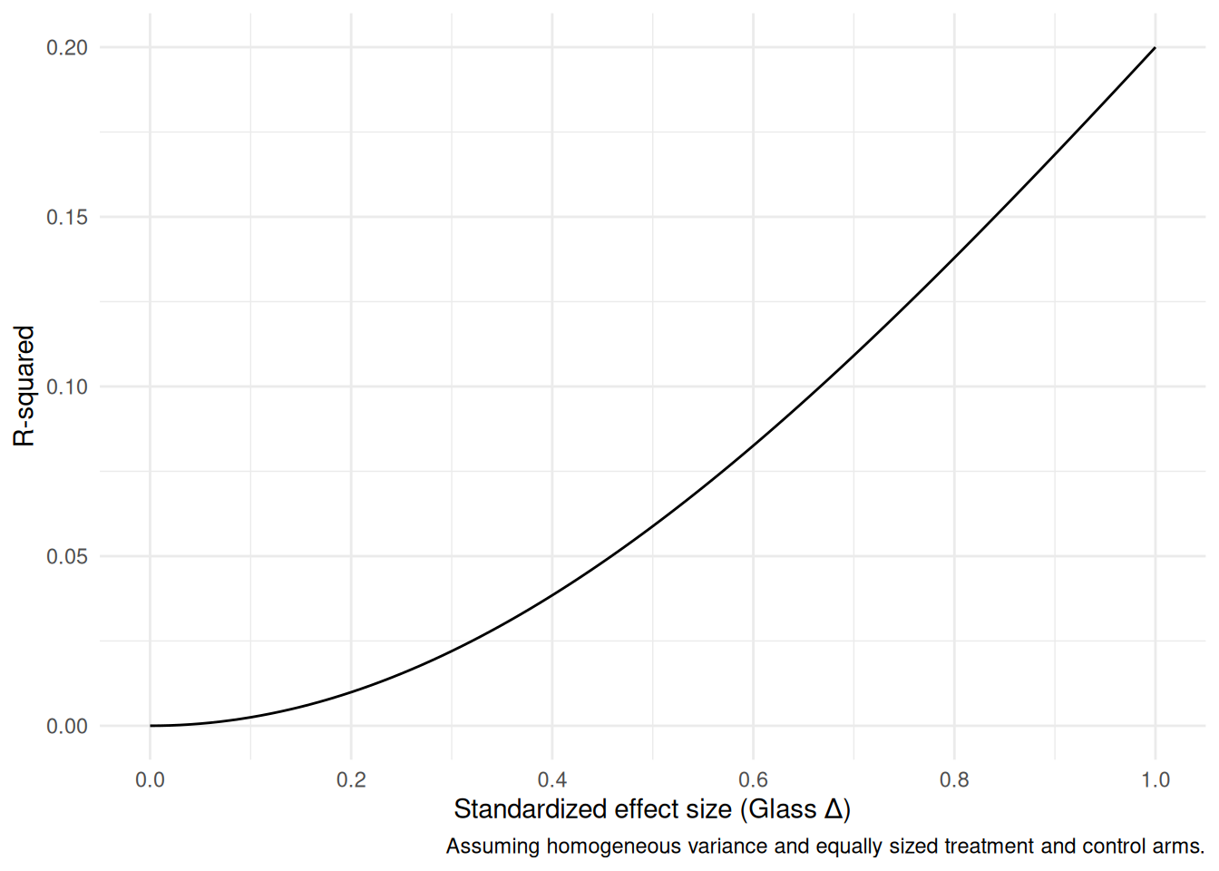
We see that even for treatment effect sizes that are quite respectable, the amount of explained variance is quite limited. For a \(0.2\sigma\) effect, \(R^2\approx 0.01\).